---

---

Artificial Music Generation

Behind the viral clips of AI-generated songs lies a very fascinating technology that's evolving at a very fast speed. While companies like Suno and Udio capture headlines with their impressive (and sometimes controversial) commercial systems, there's a whole world of open research pushing the boundaries of what's possible.

Music is incredibly complex. When we listen to a song, we process countless elements simultaneously – melody, harmony, rhythm, lyrics, emotional nuance, and more. For AI to generate convincing music, it needs to understand and somehow quantize all these elements coherently. This creates two fundamental challenges research needs to solve:

1. Big Data: Music is massively data-intensive. A typical 3-minute song at studio quality (44.1kHz) contains nearly 8 million individual data points. That's way too much raw information for even powerful AI models to process effectively - e.g. Gemini 2.5 Pro promotes an insane context window of 1.000.000 tokens, which still wouldn't be enough to process a single song of full length.
2. Musical Structure: Music isn't random. It follows patterns that span multiple time scales – from microsecond-level timbre characteristics to minute-long compositional structures. A good melody needs to make sense note-by-note while also creating a satisfying phrase over time.

In this post, I'll break down how cutting-edge AI systems are tackling these challenges through two key innovations:

• Audio Tokenization: How researchers compress massive audio files into manageable tokens that AI can understand (similar to how language models handle words)
• Generation Methodologies: The two competing approaches to creating music – autoregressive transformers vs. diffusion models

We'll look at recently published research like YuE, SongGen, X-Codec, and DiffRhythm that represent the current state-of-the-art in open music generation. Even if these specific model names are new to you, understanding their fundamental approaches will help you make sense of any AI music system you encounter.

Even if you're not planning to build your own AI music generator, understanding these foundations is valuable because:

• These same technologies are becoming available in creative tools you might use
• The strengths and limitations of each approach directly impact what kind of music they can create
• Open-source alternatives are making this technology accessible beyond big tech companies
• It is insanely fascinating to see what's possible when you combine AI with music

Ready to dive deeper? Let's start by exploring how AI systems tackle the massive data challenge through audio tokenization.

To understand why audio tokenization is necessary, we must first explore how audio is digitally represented. Digital audio is characterized by several key parameters that directly impact its dimensionality:

1. Sample Rate: Determines how many samples per second are used to represent the waveform of the audio. Standard studio-quality audio uses 44.1 kHz, meaning 44,100 samples are captured every second to represent the amplitude of the sound wave at that moment.

2. Bit Depth: Defines how many bits are used to represent each sample. Common bit depths are 16-bit (studio quality) or 24-bit (professional audio), with higher bit depths allowing for more dynamic range and precision.

3. Channels: Determines if the audio is mono (1 channel), stereo (2 channels), or a more complex format like 5.1 surround sound (6 channels).

These parameters combine to determine the bit rate of the audio, calculated as:

\(\text{Bit rate} = \text{Sample rate} \times \text{Bit depth} \times \text{Channels}\)(1)

For example, a standard stereo studio-quality recording (44.1 kHz, 16-bit, 2 channels) has a bit rate of 1,411.2 kbps. This translates to an enormous amount of data — a 3-minute song contains approximately 7,938,000 samples (44,100 × 60 × 3).

This high-dimensional representation creates a fundamental bottleneck for AI models. Even with efficient attention mechanisms, the computational complexity of transformer models scales with O(N² × D), where N is the sequence length and D is the model's hidden dimension. Processing raw audio becomes computationally prohibitive, necessitating more efficient representations.

Audio presents another unique challenge: it contains hierarchical temporal dependencies spanning multiple time scales:

• Microsecond level (20-100μs): Harmonic content and timbre characteristics
• Millisecond level (10-100ms): Phonemes in speech, individual notes in music
• Second level (1-10s): Words, musical phrases, and motifs
• Minute level (60s+): Song structure, movements, complete compositions

An effective audio representation must preserve information across all these time scales while significantly reducing dimensionality.

The solution to these challenges comes through neural network architectures that can learn lower-dimensional encodings of audio while retaining its essential characteristics. Autoencoders form the foundation of this approach.

As shown above, the autoencoder consists of three primary components:

• The encoder (E) maps the high-dimensional raw audio waveform (R^T) to a lower-dimensional latent space (Z^T')
• The latent space stores the compressed representation
• The decoder (D) reconstructs the original waveform (R^T) from this compressed form

Mathematically, this can be represented as:

• E: R^T → Z^T'
• D: Z^T' → R^T

Where T represents the original time steps and T' represents the significantly reduced token sequence length.

For audio compression, the encoder typically uses convolutional layers to capture local features, while the decoder employs transposed convolutions to reconstruct the waveform. Audio tokenizers process short frames (~20ms) rather than entire songs because it's computationally more efficient and allows the model to focus on local acoustic features while making the output compatible with sequence models context windows. This effectively allows the encoder to encode dynamic audio length by iteratively dividing an audio snippet into smaller audio frames. This is way the encoding speed of an autoencoder is also given by it's Bitrate.

While basic autoencoders can reduce dimensionality, Variational Autoencoders (VAEs) introduced by Kingma et al. organize the latent space in a way that's particularly valuable for generative tasks.

VAEs encode inputs as probability distributions rather than fixed points in the latent space. The encoder outputs:

1. A mean vector (μ) that indicates where in the latent space the encoded input is centered
2. A standard deviation vector (σ) that defines the distribution around that center

The VAE training objective optimizes the Evidence Lower Bound (ELBO):

\(L(\theta, \phi; x) = E_{q_\phi(z|x)}[\log p_\theta(x|z)] - D_{KL}(q_\phi(z|x)||p_\theta(z))\)(2)

This combines:

• A simple reconstruction term (such as MSE) that ensures accurate reproduction of the input
• The Kullback-Leibler divergence (KL-Divergence) term that encourages the encoded distributions to match a prior (typically a standard Gaussian)

The KL divergence term is crucial as it "organizes" the latent space, pushing encodings toward the origin and creating a structured, continuous representation as can be seen in this 2-dimensional visualization. This allows for meaningful interpolation between points and enables sampling from the prior distribution to generate new content.

For a more detailed explanation of VAEs and the role of KL divergence, this video provides an excellent visual breakdown.

While VAEs provide a structured latent space, they still produce continuous representations. This creates a fundamental mismatch with transformer models, which were originally designed to work with discrete tokens like words in language. Autoregressive transformers operate by predicting the next token in a sequence based on previous tokens, a task that becomes more challenging with continuous values that can vary infinitely.

The Vector Quantized-Variational AutoEncoder (VQ-VAE) introduced by van den Oord et al. addresses this issue by incorporating vector quantization into the autoencoder architecture. Instead of encoding inputs to continuous points, VQ-VAE maps them to discrete entries from a learned codebook.

The quantization process works as follows:

1. The encoder (E) produces a continuous output z_e(x) for an input x
2. This continuous vector is mapped to the nearest entry in a learned codebook of embedding vectors
3. The selected codebook entry e_k becomes the discrete representation

This can be expressed mathematically as:

\(z_q(x) = e_k \text{ where } k = \arg\min_j ||z_e(x) - e_j||^2_2\)(3)

The decoder then reconstructs the input from this quantized representation. The codebook itself is learned during training, with the model adjusting the vectors to better represent the data distribution.

This discrete representation offers two key advantages:

1. Compatibility with transformers: The indices of the selected codebook entries (k) form a discrete vocabulary that transformers can process efficiently. Each index represents a "word" in the audio language.

2. Compression efficiency: The codebook typically contains far fewer entries (e.g., 512 or 1024) than possible values in a continuous space, enabling more efficient representation.

In a standard VQ-VAE architecture, each frame of audio is encoded into a single codebook index. This index points to a vector in the codebook where each dimension represents a specific acoustic feature of that time frame. The transformer's vocabulary then consists of these indices, with each "token" representing a compressed timeframe audio segment.

While basic VQ-VAE provides a discrete representation, achieving high-fidelity audio often requires more detailed encoding than a single codebook vector can provide. Residual Vector Quantization (RVQ) addresses this limitation by applying vector quantization in multiple stages, significantly improving audio quality while maintaining transformer compatibility.

RVQ works through an iterative quantization process:

1. The first quantizer Q₁ maps the encoder output z_e(x) to the nearest vector in the first codebook, producing z_q⁽¹⁾

2. Rather than stopping there, RVQ calculates the residual (the error between the original encoding and the quantized version): r⁽¹⁾ = z_e(x) - z_q⁽¹⁾

3. This residual is then quantized by a second codebook Q₂, producing z_q⁽²⁾

4. The process continues for N_q stages, with each subsequent codebook capturing finer details missed by previous quantizations

The final representation consists of a sequence of codebook indices (k₁, k₂, ..., k_Nq) from each quantization step. Conceptually, the first codebook captures the overall structure of the audio frame, while subsequent residual codebooks refine the details, similar to how JPEG compression works for images.

This approach offers significant advantages:

1. Higher compression ratios: RVQ achieves better audio fidelity at comparable bitrates compared to single-codebook approaches

2. Controllable quality-size tradeoff: By using more or fewer codebooks during inference, models can adjust the fidelity/compression ratio

3. Expanded transformer vocabulary: The vocabulary expands to codebook_size × num_codebooks, with each unique combination of indices representing a specific audio configuration

The transformer's vocabulary now consists of these combined indices, where each token represents both the primary acoustic features (codebook 0) and their refinements (residual codebooks 1 to N). During generation, the transformer predicts these indices sequentially, which are then mapped back to the corresponding codebook vectors and combined to reconstruct the audio.

Standard audio codecs like EnCodec and RVQ-GAN focus primarily on acoustic fidelity—preserving the sound quality as accurately as possible. However, they often neglect the semantic meaning within audio (like the words spoken, musical structure, or instrument identification). This creates a challenge for downstream Large Language Models (LLMs) that must infer these meanings from purely acoustic tokens.

X-Codec, developed by Ye et al., addresses this limitation through an innovative "X-shaped" architecture that directly embeds semantic information into the audio tokens. This approach makes it substantially easier for models like YuE to understand and process the audio content.

The pipeline of X-codec

The X-Codec architecture works through several key mechanisms:

1. Dual-Stream Processing: Unlike traditional codecs that process only acoustic features, X-Codec processes two parallel streams:

   • An acoustic stream that captures the sound quality (using standard audio processing)
   • A semantic stream that extracts high-level features using a pre-trained self-supervised model (like HuBERT)

2. Unified Representation: These two streams are combined into a single latent representation before quantization, creating tokens that contain both acoustic and semantic information

3. Standard RVQ: This unified representation is then quantized using a standard Residual Vector Quantizer, making it compatible with existing Audio LLM architectures

4. Dual Reconstruction Objective: During training, X-Codec is required to reconstruct both:

   • The original audio waveform (acoustic reconstruction)
   • The initial semantic features (semantic reconstruction)

This approach provides several significant advantages:

1. Improved Lyrical Coherence: By preserving semantic information in the tokens themselves, models like YuE achieve much better word error rates and lyrical coherence

2. Better Phonetic Discriminability: The internal representations become much better at distinguishing between similar phonetic sounds

3. Balanced Performance: X-Codec manages to improve semantic capability while maintaining or improving speaker similarity and audio naturalness

X-Codec represents a key innovation in audio tokenization, directly addressing a fundamental bottleneck in music generation by making it easier for language models to work with the semantic content of audio. Models like YuE that leverage X-Codec can follow lyrics more accurately and maintain better musical structure throughout a composition.

Now that we have a powerful way to represent short timeframes of audio space in the latent space, we need powerful models to generate these tokens (our codebook indices) in coherent sequences that form musical compositions. Two main architectural paradigms have emerged in recent research: autoregressive transformers and diffusion-based models. Let's examine each approach, starting with the more established autoregressive method.

Autoregressive models represent the cornerstone of sequence generation, operating on a simple yet powerful principle: predict the next token based on all previous tokens. This approach inherently captures temporal dependencies - crucial for music where each note or sound should logically follow from what came before.

Mathematically, autoregressive models calculate the probability of a token sequence as a product of conditional probabilities:

\(p(z) = \prod_{i=1}^{n} p(z_i|z_{<i})\)(3)

Where each token (z₁) is predicted based on all previous tokens (z₍₁). This sequential generation process has historically excelled at maintaining musical coherence and precise timing, making it particularly well-suited for following musical structures like verses, choruses, and bridges.

A prime example of state-of-the-art autoregressive music generation is YuE, an open foundation model family based on the LLaMA2 architecture. YuE demonstrates how autoregressive approaches can be scaled and enhanced to generate high-quality music with vocals and accompaniment for durations up to five minutes.

YuE employs a two-stage approach:

1. Stage 1: A large language model generates the basic musical structure (codebook-0 tokens) using semantically-rich tokens from X-Codec.
2. Stage 2: A smaller model (1B parameters) refines the acoustic details (codebook 1-7) by predicting residual codebooks for higher fidelity.

This separation allows YuE to maintain coherence over extended durations while still capturing fine acoustic details. But what makes YuE truly innovative are three architectural contributions that directly address historical limitations of autoregressive music generation:

Traditional autoregressive models struggle when generating mixed audio (vocals + accompaniment) because vocals often become unintelligible, especially in dense music like metal. YuE's solution is elegantly simple yet effective:

Instead of generating a single token (xₜ) at each timestep that represents the mixed audio, YuE explicitly predicts two separate tokens:

• A vocal token (vₜ)
• An accompaniment token (aₜ)

The model's sequence then becomes:

\((v_1, a_1, v_2, a_2, ..., v_T, a_T)\)(4)

This approach allows both tracks to influence each other while being processed separately, significantly reducing the word error rate in the vocal track. The probability factorizes as:

\(p(v_t, a_t|v_{<t}, a_{<t}; \theta) = p(v_t|v_{<t}, a_{<t}; \theta) \times p(a_t|v_{\leq t}, a_{<t}; \theta)\)(5)

By breaking the prediction into these two components, YuE maintains the clarity of vocals even in musically dense sections.

How do you maintain lyrical coherence over thousands of tokens? Standard transformer models with common positional embeddings like RoPE struggle beyond about 3,000 tokens, leading to the model "forgetting" lyrics or structure in longer pieces.

YuE's structural progressive conditioning elegantly addresses this through a segmented approach to song generation. The model explicitly divides songs into natural musical structures (verse, chorus, bridge) and interleaves text and audio tokens segment by segment:

\(s_i = [SOS] \circ \tau_i \circ \ell_i \circ <SOA> \circ \psi_i \circ <EOA> \circ [EOS]\)(6)

Where:

• <SOS>/<EOS>: Start/End of Segment markers
• τᵢ: A structure label (e.g., [verse], [chorus])
• ℓᵢ: The segment's lyrics
• <SOA>/<EOA>: Start/End of Audio markers
• ψᵢ: The corresponding Dual-NTP audio tokens

This structure provides constant reminders of lyrical context throughout generation, essentially giving the model signposts to follow as it generates longer pieces.

Style control is crucial for creative music generation. YuE enables reference-guided generation by prepending 20-40 seconds of audio tokens from an existing song to the generation structure.

This allows for impressive creative control:

• Zero-shot voice cloning (copying a singer's voice without training)
• Style transfer (transforming genres while preserving content, like Japanese city pop into English rap)
• Instrumental style matching

To prevent the model from simply copying reference audio, YuE employs a delayed activation strategy during training. The ~40 billion tokens of ICL data are only introduced during the final training stage, after the model has already learned to generate music independently.

While YuE demonstrates the power of complex autoregressive architectures, SongGen shows that simpler, more streamlined approaches can also achieve impressive results. Unlike YuE's two-stage process, SongGen uses a single-stage autoregressive transformer for text-to-song generation.

The model offers two flexible output modes:

1. Mixed Mode: A single audio track with blended vocals and accompaniment
2. Dual-Track Mode: Separate but synchronized vocal and accompaniment tracks

At its core, SongGen uses a 24-layer transformer decoder that processes three inputs:

• Tokenized lyrics (using VoiceBPE)
• Descriptive text for style (using T5)
• An optional 3-second reference voice clip (encoded with MERT)

These inputs are incorporated via cross-attention mechanisms, with X-Codec handling audio tokenization (using 8 codebooks).

Like YuE, SongGen identified the challenge of vocal clarity in mixed audio. Their solution, "Mixed Pro," introduces an auxiliary loss term during training:

\(L_{mixed-pro} = L_{mixed} + \lambda L_{vocal}\)(7)

By separating original songs into isolated vocal and accompaniment tracks using Demucs, SongGen creates training data that enables the model to simultaneously predict both mixed and vocal-only tokens. This significantly improves vocal intelligibility without requiring architectural changes during inference.

The contrast between YuE's sophisticated two-stage approach and SongGen's streamlined single-stage design highlights important architectural trade-offs in autoregressive music generation:

• Complexity vs. Efficiency: YuE's architecture enables more detailed control and higher acoustic quality but requires more computational resources. SongGen achieves competitive results with lower requirements and simpler implementation.

• Scale vs. Innovation: YuE leverages the proven scaling properties of large language models (demonstrating models up to 7B+ parameters), while SongGen shows that architectural innovations can sometimes compensate for raw model size.

• Generation Speed: Both approaches share a fundamental limitation - as autoregressive models, generation speed scales linearly with sequence length. A 5-minute song requires many sequential steps, making real-time generation challenging.

This last limitation has motivated researchers to explore alternative non-autoregressive approaches that could maintain musical quality while addressing the efficiency bottleneck. In the next section, we'll explore diffusion-based models, which offer a radically different approach to sequence generation with promising advantages in generation speed.

While autoregressive models have dominated sequence generation, they face a fundamental limitation: generation speed. For longer pieces, prediction time increases linearly with sequence length, making real-time generation of full songs challenging. This constraint has motivated researchers to explore a radically different approach: diffusion models.

Diffusion models work by reversing a gradual noising process. Instead of predicting one token at a time based on previous tokens, diffusion starts with pure random noise and iteratively refines it over a series of steps until a clean, coherent audio sample emerges:

\(z_{t-1} \sim p_\theta(z_{t-1}|z_t)\)(8)

A key distinction between autoregressive and diffusion approaches lies in how they represent the latent space. While autoregressive models excel with discrete tokens (like those from X-Codec), diffusion models fundamentally require continuous vector spaces. Here's why:

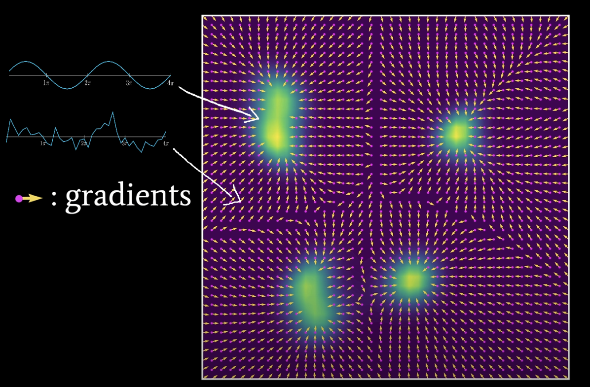
Diffusion models operate by gradually denoising data from random Gaussian noise. This denoising process relies on smooth gradients to guide the transformation from noise to structure. Discrete tokens create discontinuities in this space - imagine trying to draw a smooth curve through a series of isolated points versus a continuous line.

In a VAE's continuous latent space, each timeframe of audio is represented as an n-dimensional vector (typically 256 to 1024 dimensions). These vectors occupy a smooth manifold where similar sounds have similar vector representations, enabling gradual transformations through the diffusion process.

During diffusion:

1. We start with a sequence of completely random vectors (z_T) - one for each timeframe
2. These vectors have the same dimensionality as our latent space (e.g., 512-dimensional vectors)
3. Each denoising step slightly adjusts these vectors toward more "musical" configurations
4. After many iterations, we arrive at a sequence of vectors (z₀) that represent coherent music

This process can be seen as traversing a probability landscape, gradually moving from high-entropy random states toward lower-entropy structured states that represent valid sounds or music.

Using continuous representations offers several advantages for diffusion models:

1. Smoother Denoising Gradients: Continuous spaces provide well-defined gradients everywhere, allowing for more stable and effective denoising steps. Discrete tokens would create "jumps" in the probability space.

2. Richer Acoustic Detail: Continuous representations can preserve more fine-grained acoustic details compared to the information bottleneck of discrete codebooks, potentially allowing for higher fidelity.

3. Interpolation Capabilities: Points between valid discrete tokens can represent meaningful intermediate sounds, enabling more nuanced control over generation.

4. Parallel Computation: Most importantly, the entire sequence can be processed simultaneously during each denoising step, rather than generating one token at a time.

This last point is crucial. Instead of autoregressively generating thousands of tokens sequentially, diffusion models apply a series of denoising steps to the entire sequence in parallel. While each step must still be performed sequentially, the number of steps (typically 50-100) is usually far fewer than the number of tokens in a musical sequence (thousands for a typical song).

A notable implementation of this approach is DiffRhythm, presented as the first open-source model to apply a full diffusion process to song generation. DiffRhythm can synthesize complete stereo songs with both vocals and accompaniment for durations approaching five minutes in just about ten seconds - dramatically faster than autoregressive alternatives.

DiffRhythm's architecture comprises three main components:

1. Latent Representation via VAE: Rather than using discrete tokens, DiffRhythm employs a continuous latent space through the Stable Audio Open tokenizer. The encoder (E) compresses raw audio waveforms into a compact latent sequence, while the decoder (D) reconstructs audio from generated latent vectors.

2. Diffusion Transformer (DiT): The core generative component operates entirely within this compressed latent space. Instead of the U-Net architecture common in image diffusion, DiffRhythm implements a Diffusion Transformer (DiT) based on LLaMA-2 decoder layers. The DiT works by:

   • Dividing the latent sequence into "patches" with N dimensions at each position
   • Treating these patches as a sequence of vectors fed into standard transformer blocks
   • Learning a step-by-step denoising process that gradually transforms random noise into coherent music

3. Training with Flow Matching: To train the DiT efficiently, DiffRhythm uses conditional Flow Matching. This approach trains the model to predict the optimal path or velocity needed to transform random noise toward a target latent representation learned from training data.

To understand how DiffRhythm generates music, let's walk through the process:

1. Initialization: Start with a sequence of random Gaussian noise vectors z_T representing each timeframe in the latent space.

2. Conditioning: The model incorporates conditioning information like lyrics (aligned at the sentence level) and a style reference audio clip.

3. Iterative Denoising: The DiT applies a series of denoising steps (typically 50-100), gradually transforming the random vectors toward musically coherent structures:

   • Each step takes the entire sequence as input
   • The transformer's self-attention allows distant timeframes to influence each other
   • The model predicts the direction to move each vector to reduce noise
   • After each step, the sequence becomes more structured and coherent

4. Waveform Generation: Once denoising is complete, the final latent representation z₀ is passed through the VAE decoder to reconstruct the full audio waveform.

The critical advantage lies in processing the entire sequence in parallel at each step - even for a 5-minute song. While autoregressive models must generate each token one after another (potentially thousands of sequential operations), diffusion models can simultaneously update every timeframe in the sequence during each denoising step.

DiffRhythm demonstrates that diffusion-based approaches can offer dramatically faster inference speeds compared to autoregressive models (claiming a 10-50x speedup). This makes them particularly attractive for applications requiring near-real-time generation or interactive creative workflows.

However, this speed comes with trade-offs. Current autoregressive models like YuE still tend to produce more coherent lyrics and complex musical structures, particularly for extended compositions with multiple sections. This makes sense intuitively - autoregressive models explicitly condition each token on all previous tokens, which naturally captures long-range dependencies and structural patterns.

Diffusion models must capture these dependencies through the transformer's self-attention mechanism across denoising steps. While this works well for local coherence and many musical elements, precisely following complex structural patterns like verse-chorus relationships remains challenging.

DiffRhythm addresses this through a simpler but robust lyrics alignment strategy, using sentence-level anchoring rather than word-level precision. This pragmatic approach trades some fine-grained control for dramatically improved generation speed.

The contrast between autoregressive and diffusion approaches illustrates a key tension in music generation:

• Autoregressive Models (YuE, SongGen) excel in control and temporal precision but are fundamentally limited in generation speed.

• Diffusion Models (DiffRhythm) offer dramatically faster generation through parallel computation but may sacrifice some fine-grained structural control.

Both approaches continue to evolve rapidly, with researchers working to address their respective limitations. The ideal music generation system might eventually combine elements of both paradigms - perhaps using diffusion for initial generation and autoregressive refinement for structural coherence, or developing hybrid architectures that leverage the strengths of each approach.

What's clear is that these complementary research directions are pushing the boundaries of what's possible in AI music generation, bringing us closer to systems that can generate high-quality, diverse musical compositions with unprecedented speed and flexibility.

I hope this article has provided you a good overview of the current state in the field of artificial music generation. This is definetly one of the most interesting research areas to me so feel free to contact me if you have any questions or might even want to start a collaboration. I am always open to new ideas and projects :)