The previous post built the Fourier transform: a signal is a sum of pure oscillations, and the transform recovers the amplitude and phase of each one. This post uses that machinery to build an actual architecture. The Fourier Neural Operator (FNO) is a neural operator in the sense of Post 7 — it approximates the solution operator of a PDE, and it attaches its weights to resolution-independent objects rather than to grid points. In FNO those objects are frequency modes.

The post starts from the problem FNO exists to solve, then walks through every layer of the architecture in the order data flows through it, tracking the tensor shape at each step.

A convolution takes a short list of numbers, called the kernel, and slides it along a longer list, computing one weighted sum per position.

\(o_i = \sum_{m=-r}^{r} k_m \, s_{i+m}\)(1)

Where \(s\) denotes the input signal as a list of numbers, \(s_{i+m}\) denotes its entry at index \(i+m\), \(k_m\) denotes the kernel weight at offset \(m\), \(r\) denotes the kernel's half-width (so a three-entry kernel has \(r = 1\) and offsets \(m \in \{-1, 0, 1\}\)), and \(o_i\) denotes the output at index \(i\).

Take the kernel \(k = [1, -2, 1]\) and the signal \(s = [2, 5, 3, 8, 1]\). To compute the output at index 2, center the kernel on \(s_2 = 3\) and take the weighted sum of that entry and its two neighbours.

\(o_2 = 1 \cdot 5 + (-2) \cdot 3 + 1 \cdot 8 = 5 - 6 + 8 = 7\)(2)

Where the three products pair the kernel weights \(k_{-1} = 1\), \(k_0 = -2\), \(k_1 = 1\) with the signal entries \(s_1 = 5\), \(s_2 = 3\), \(s_3 = 8\), and \(o_2\) denotes the resulting output value at index 2.

That kernel is not arbitrary. It is Post 2's three-point curvature stencil \((u_{i+1} - 2u_i + u_{i-1})/\Delta x^2\) without the division by \(\Delta x^2\), where \(u_i\) denotes the field value at grid point \(i\) and \(\Delta x\) denotes the grid spacing. Every finite-difference update in Posts 2 through 6 was a convolution. A convolutional layer in a neural network performs the same operation, with the kernel entries learned from data instead of derived from the second derivative stencil.

A kernel of half-width \(r\) combines a point with \(r\) neighbours on each side — a total of \(k = 2r+1\) points. Track what a single output value has "seen" as more of these layers stack, working through \(k=3\) (so \(r=1\)) one layer at a time.

Layer 0 — the raw input. Point \(i\) has seen only itself.

Layer 1 — one convolution applied. Point \(i\)'s new value is a weighted sum of \(i-1, i, i+1\). It has now seen 3 original input points.

Layer 2 — a second convolution applied to layer 1's output. Point \(i\)'s new value combines three layer-1 values, not three raw inputs: its own layer-1 value (which already saw \(i-1,i,i+1\)), its left neighbour's layer-1 value at \(i-1\) (which already saw \(i-2,i-1,i\)), and its right neighbour's layer-1 value at \(i+1\) (which already saw \(i,i+1,i+2\)). Taking the union of those three ranges, point \(i\) has now seen \(i-2\) through \(i+2\) — width 5.

Generalizing this growth pattern across \(L\) layers gives the receptive field: the number of input positions that can influence a single output position after \(L\) layers.

\(R(L) = 1 + L(k-1)\)(3)

Where \(R(L)\) denotes the receptive-field width in grid points, \(L\) denotes the number of stacked convolutional layers, and \(k\) denotes the kernel width in grid points as defined above. Checking it against the two layers just worked through: \(R(1) = 1 + 1\cdot 2 = 3\) matches layer 1's width of 3, and \(R(2) = 1 + 2\cdot 2 = 5\) matches layer 2's width of 5.

Now put a number on it. For a domain discretized into 1000 grid points, connecting one end to the other requires \(R(L) \geq 1000\), so \(1 + 2L \geq 1000\), so roughly 500 layers. That is the cost of building global reach out of local, neighbour-only operations.

This matters directly for the wave equation. Post 6 established that information propagates at speed \(c\), and that a stable explicit solver must respect the CFL condition \(c\Delta t \leq \Delta x\), where \(c\) denotes wave speed, \(\Delta t\) denotes the time step and \(\Delta x\) denotes grid spacing. A network that has to reproduce a large time step in one forward pass needs a wavefront to move many grid cells at once, and a stack of small kernels can only deliver that with enormous depth.

Post 8 gave the discrete Fourier transform.

\(S_k = \sum_{i=0}^{N-1} s_i \, e^{-j 2\pi k i / N}\)(4)

Where \(S_k\) denotes the complex coefficient of mode \(k\), \(s_i\) denotes the signal sample at grid index \(i\), \(N\) denotes the number of samples, \(k\) denotes how many full oscillations the reference wave completes across the whole sampled domain, and \(j\) denotes the imaginary unit with \(j^2 = -1\).

Every sample \(s_i\) appears in that sum. A single coefficient is already a global summary of the field. Editing it and transforming back changes the field everywhere. That is the entire motivating idea of the Fourier Neural Operator: perform the layer's mixing step on coefficients rather than on grid neighbourhoods, and one layer reaches the whole domain.

Post 8 established the mechanism; this section only fixes the reading of the two numbers stored per mode, because the architecture manipulates them directly.

Expanding the reference wave with Euler's formula splits the sum into two real sums.

\(S_k = \underbrace{\sum_{i=0}^{N-1} s_i \cos(2\pi k i / N)}_{\text{real part } x} \; - \; j \underbrace{\sum_{i=0}^{N-1} s_i \sin(2\pi k i / N)}_{\text{imaginary part magnitude } y}\)(5)

Where \(x\) denotes the real part of \(S_k\), measuring how strongly the signal resembles a cosine at mode \(k\), and \(y\) denotes the sine similarity, which enters the coefficient with a minus sign so that \(S_k = x - jy\); the other symbols are as above.

The two numbers can be read either as a pair or in polar form. The magnitude \(|S_k| = \sqrt{x^2 + y^2}\) is the amplitude of that oscillation in the signal, and the angle \(\arg(S_k)\) is its phase — where the oscillation's peak sits relative to the origin. Both symbols are as defined above.

Check this on a signal that is exactly one cosine. Take \(s = [1, 0, -1, 0]\) with \(N = 4\), which is \(\cos(2\pi i / 4)\) sampled at \(i = 0,1,2,3\), and evaluate mode \(k = 1\). The reference wave takes the values \(1, -j, -1, j\) at those four indices.

\(S_1 = 1 \cdot 1 + 0 \cdot (-j) + (-1)\cdot(-1) + 0 \cdot j = 2 + 0j\)(6)

Where \(S_1\) denotes the coefficient of mode 1, the first factor in each product is the signal sample \(s_i\) and the second is the reference-wave value \(e^{-j2\pi i/4}\) at that index.

The result is the pair \((2, 0)\): all cosine similarity, no sine similarity, phase zero. The magnitude 2 equals the signal's amplitude of 1 times \(N/2\), the standard scaling of the unnormalized transform.

The concrete problem for the rest of this post is one step of the wave equation's solution operator in two spatial dimensions. Post 4 established that the wave equation needs a two-field state: the displacement field \(U\) and the velocity field \(V = \partial U/\partial t\), where \(t\) denotes time. A single snapshot of displacement alone cannot determine the next state.

Discretize the domain on a 100 by 100 grid. The input to the network is then a tensor of shape (2, 100, 100): two channels, one per field, each holding a 100 by 100 array of grid values. A channel is a full spatial field; a grid cell holds one number per channel. At the very start, the two numbers at a given cell are that cell's displacement and velocity.

Every operation below is stated twice: what it does to the tensor shape, and what it does to the numbers sitting at one individual grid cell.

The first layer is a lifting layer: a linear map applied independently at every grid cell, which increases the channel count.

\(v(x) = P\, a(x) + p\)(7)

Where \(a(x)\) denotes the input channel vector at grid position \(x\) (here the two numbers \((U, V)\) at that cell), \(P\) denotes a learnable weight matrix of shape (4, 2), \(p\) denotes a learnable bias vector of length 4, and \(v(x)\) denotes the resulting lifted vector of 4 numbers at the same position.

Take a cell whose values are \((U, V) = (3, -2)\) and a weight matrix

\(P = \begin{bmatrix} 1 & 0 \\ 0 & 1 \\ 1 & 1 \\ 1 & -1 \end{bmatrix}\)(8)

Where each row of \(P\) produces one output channel, and the two entries in a row are the weights applied to the displacement and the velocity respectively. Taking the bias to be zero:

\(P \begin{bmatrix} 3 \\ -2 \end{bmatrix} = \begin{bmatrix} 1\cdot 3 + 0\cdot(-2) \\ 0\cdot 3 + 1\cdot(-2) \\ 1\cdot 3 + 1\cdot(-2) \\ 1\cdot 3 + (-1)\cdot(-2) \end{bmatrix} = \begin{bmatrix} 3 \\ -2 \\ 1 \\ 5 \end{bmatrix}\)(9)

Where the input column vector holds the cell's displacement and velocity, and the output column vector holds the four lifted values at that cell.

The same matrix \(P\) is applied at all 10,000 cells, so the tensor shape goes from (2, 100, 100) to (4, 100, 100).

Two channels are too narrow to carry the intermediate representation. The layers that follow mix channels together, and with only two channels there are just four mixing coefficients available per frequency mode — far too few to represent a useful learned transformation. Widening also breaks the interpretation: after lifting, the four numbers at a cell are learned features, not displacement and velocity. Nothing forces channel 1 to remain \(U\). Real implementations lift to 32 or 64 channels; 4 is used here so the arithmetic stays writable.

Because the lifting map is the same at every position and involves no neighbours, it is resolution independent in the sense of Post 7: the same weights apply on a grid of any size.

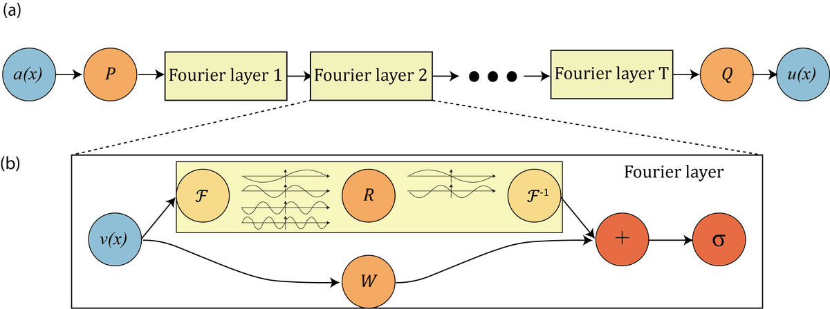
The lifted tensor now enters the core of the architecture. An FNO block splits into two parallel paths. The spectral branch is the global one, and it runs in four steps.

Each of the 4 channels is transformed independently with a two-dimensional discrete Fourier transform. Post 8 gave the two-dimensional reference wave; the transform is the same dot-product-against-a-reference-wave construction, now with a frequency index per axis.

\(\hat{v}(k_1, k_2) = \sum_{i=0}^{N_1-1} \sum_{l=0}^{N_2-1} v_{i,l} \, e^{-j2\pi\left(\frac{k_1 i}{N_1} + \frac{k_2 l}{N_2}\right)}\)(10)

Where \(\hat{v}(k_1,k_2)\) denotes the complex coefficient of the two-dimensional mode \((k_1, k_2)\) for one channel, \(v_{i,l}\) denotes that channel's value at grid cell \((i, l)\), \(N_1\) and \(N_2\) denote the grid size along each axis (both 100 here), \(k_1\) denotes the number of oscillations across the first axis, \(k_2\) the number across the second, and \(j\) the imaginary unit.

A naive implementation would produce a 100 by 100 array of complex coefficients per channel. Half of that is redundant. The input field is real-valued, and for real input the coefficients obey a conjugate symmetry.

\(\hat{v}(-k_1, -k_2) = \overline{\hat{v}(k_1, k_2)}\)(11)

Where the overline denotes complex conjugation, meaning the real part is unchanged and the imaginary part flips sign, and \((-k_1, -k_2)\) denotes the mode with both frequency indices negated.

The reason is that a real signal has no imaginary content to encode, so the negative-frequency half carries no new information: the sine similarity at mode \(-k\) is exactly minus the sine similarity at mode \(+k\), and the cosine similarities are equal. This is the same statement as the sampling limit: \(N\) real samples carry exactly \(N/2 + 1\) independent frequencies, running from the constant mode \(k = 0\) up to the Nyquist mode \(k = N/2\), the fastest oscillation the grid can represent — one full period every two grid points.

The Real-Values FFT exploits this by returning only the non-redundant half along the last axis. For a 100 by 100 field that is 51 columns, since \(100/2 + 1 = 51\). The tensor is now (4, 100, 51), holding one complex number per channel per mode. This can honestly trip you up a bit, so I encourage you to make a deep dive into this topic, even though it is not necessary. Just remember, that our input value has no imaginary part. Throwing the signal into the DFT produces complex coefficients. However, the imaginary part does not contain any new information. Therefore, for the output signal to be real again, the imaginary parts of the coefficients must be conjugate symmetric for the imaginary parts to cancel out.

The next step discards most of those modes. Fix a mode count \(M\) per axis and keep only the lowest \(M\) frequencies; take \(M = 10\). The kept block has shape (4, 20, 10).

The asymmetry between 20 and 10 comes from the folding in Step 1. The second axis was folded, so its negative frequencies are already gone and keeping the 10 lowest means 10 columns. The first axis was not folded, so it still stores both signs: its 100 rows run from mode 0 upward through the Nyquist mode and then continue as the negative modes counting back toward \(-1\). Keeping the 10 lowest in each direction means 10 rows from the top of the array and 10 from the bottom, hence 20.

Low modes are kept because they carry almost all of a field's shape: the coarse structure holds most of the amplitude, and coefficient magnitudes decay as frequency rises.

The more important property is what a fixed mode count buys. Mode 7 names a shape — a wave that repeats 7 times across the whole domain — not a grid location. Sample that shape with 100 points or with 400 and it is still the same 7 repetitions, just measured more finely. So a weight attached to mode 7 stays attached to the same physical wave regardless of resolution, unlike a weight attached to "grid point 7," which points somewhere different at every resolution. That is why keeping the lowest \(M\) modes always costs the same \(M\) weights, with no dependence on the grid size — the discretisation invariance of Post 7, and the reason FNO counts as a neural operator rather than a resolution-locked network.

The cost is just as direct. Keep only 10 modes, and mode 11 upward is gone, not approximated. A sharp wavefront is made of exactly those discarded modes reinforcing each other at one spot and cancelling everywhere else; remove them and the edge slumps into a slope. Post 3's heat equation was going to smooth itself anyway, so this costs it nothing. The wave equation exists to keep its edges sharp, so the same cut fights the physics directly — FNO's known weak point on hyperbolic problems.

Each kept coefficient is multiplied by a learnable complex number. Writing the coefficient as \(x + yj\) and the weight as \(a + bj\), expand the product and use \(j^2 = -1\):

\((x + yj)(a + bj) = xa + xbj + yaj + ybj^2 = (xa - yb) + (xb + ya)j\)(12)

Where \(x\) and \(y\) denote the real and imaginary parts of the coefficient, \(a\) and \(b\) denote the real and imaginary parts of the learnable weight, and \(j\) denotes the imaginary unit.

The result is two real numbers computed from four real numbers. No complex data type is required: store the real and imaginary parts as two separate real tensors and apply the formula above. Autodifferentiation then works exactly as in any real-valued network.

Geometrically, multiplying by \(a + bj\) scales the coefficient's magnitude by \(\sqrt{a^2+b^2}\) and rotates its phase by \(\arg(a+bj)\), where both symbols are as defined above. In the language of Section 2: the amplitude of that oscillation is rescaled and its peak is shifted.

This is a familiar object. Post 5 derived the growth factor \(G(\kappa)\) for the heat equation, a single number per mode by which that mode's amplitude is multiplied at every time step. Post 6 derived the eigenvalues \(\lambda\) of the amplification matrix \(M(\kappa)\) for the wave equation, complex numbers of magnitude 1 in the stable regime, which rotate a mode's phase without changing its amplitude. In both cases one step of the update acts on each Fourier mode as a single complex multiplication. FNO's spectral weights perform the same operation with one change: the multiplier is learned from data instead of derived from a known update rule. Where \(G(\kappa)\) and \(\lambda\) follow from the PDE and the chosen scheme, \(a + bj\) follows from gradient descent on training data.

Channels have not been handled yet. A single complex number per mode would process each of the 4 channels in isolation. Channel mixing follows the same rule as an ordinary convolutional layer: each output channel is a sum over all input channels, and this sum is repeated once per output channel.

\(\hat{w}_o(k_1,k_2) = \sum_{i=1}^{c_{\text{in}}} R_{o,i,k_1,k_2} \; \hat{v}_i(k_1,k_2)\)(13)

Where \(\hat{w}_o(k_1,k_2)\) denotes the output coefficient of channel \(o\) at mode \((k_1,k_2)\), \(\hat{v}_i(k_1,k_2)\) denotes the input coefficient of channel \(i\) at that same mode, \(R_{o,i,k_1,k_2}\) denotes the learnable complex weight connecting input channel \(i\) to output channel \(o\) at that mode, and \(c_{\text{in}}\) denotes the number of input channels.

The weight tensor therefore has shape (out_ch, in_ch, 20, 10), which in the running example is (4, 4, 20, 10). Counting real numbers: \(4 \times 4 \times 20 \times 10 \times 2 = 6400\) parameters, the final factor of 2 covering the real and imaginary part of each weight.

The two trailing axes of that shape carry the essential point: the weights are not shared across modes. Every one of the 200 kept modes has its own independent 4 by 4 complex matrix. This is what allows the layer to treat frequencies differently — damping one band, rotating another, leaving a third untouched. Sharing a single matrix across all modes would force the same multiplier everywhere and collapse the layer to a uniform rescaling.

The multiplied block has shape (4, 20, 10), but the inverse transform expects a full coefficient array of shape (4, 100, 51). The block is written back into an array of zeros at the mode positions it came from, and every discarded position stays zero.

This padding happens in frequency space, before the inverse transform. It does not restore the discarded content; it states that the model's output has no content at those frequencies. The inverse transform then returns to the grid, producing shape (4, 100, 100). The output of the spectral branch is a bandlimited field: a field whose Fourier content is confined to the kept modes, by construction.

Running alongside the spectral branch is a second path applied to the same lifted input. It is a linear map applied at each grid cell independently, with no neighbours involved — a 1 by 1 convolution.

Illustrate with two channels for readable arithmetic. Take the weight matrix and a cell holding \((3, 5)\):

\(W = \begin{bmatrix} 2 & 0 \\ 1 & 1 \end{bmatrix}, \qquad W\begin{bmatrix} 3 \\ 5 \end{bmatrix} = \begin{bmatrix} 2\cdot 3 + 0 \cdot 5 \\ 1 \cdot 3 + 1 \cdot 5 \end{bmatrix} = \begin{bmatrix} 6 \\ 8 \end{bmatrix}\)(14)

Where \(W\) denotes the learnable local weight matrix, the input column vector holds the channel values at one grid cell, and the output column vector holds that cell's transformed channel values. In the running example \(W\) is 4 by 4, holding 16 weights.

The same \(W\) is used at every one of the 10,000 positions, and the shape stays (4, 100, 100).

This branch reads the untruncated input. The spectral branch saw only 200 modes; the local branch sees the field as it actually is at each cell, including whatever high-frequency content the truncation removed. It is therefore the one route by which fine detail can reach the block's output. Its limitation is equally sharp: being pointwise, it can only pass a cell's own values forward, transformed. It cannot combine a cell with its neighbours, so it cannot repair a smoothed gradient — it can only carry per-cell magnitude past the cutoff.

The obvious question is why this branch is not a 3 by 3 convolution, which would at least see neighbours. The answer is resolution invariance. A 3 by 3 kernel spans a fixed number of grid cells, not a fixed physical distance. On a unit-length domain with 100 points, \(\Delta x \approx 0.01\) and the kernel reaches about \(0.02\) in physical units; on the same domain with 400 points it reaches about \(0.005\), a quarter of the footprint, where \(\Delta x\) denotes grid spacing. The same learned weights would then implement a different physical operation at each resolution, which is exactly the property FNO's mode-indexed weights were built to avoid.

Hybrids that attach a U-Net to the FNO block do recover local detail and measurably improve sharp-feature accuracy, but they lose resolution invariance at their downsampling and upsampling steps, which are counted in grid cells for the same reason. The trade is acknowledged and currently unresolved. The direction a fix would take is to define the local operation as a continuous kernel function evaluated at the actual grid spacings \(\Delta x\) and \(\Delta y\), where these denote the physical spacing along each axis, rather than as a fixed count of cells — so that refining the grid samples the same kernel more finely instead of shrinking its reach. This is an open problem, and nothing here settles it.

The two branches produce tensors of identical shape (4, 100, 100), and are combined by elementwise addition followed by a pointwise nonlinearity. That is the complete FNO block.

\(v_{\ell+1}(x) = \sigma\Big( W v_\ell(x) + b + \mathcal{F}^{-1}\big( R \cdot \mathcal{F}(v_\ell) \big)(x) \Big)\)(15)

Where \(v_\ell(x)\) denotes the channel vector at position \(x\) entering block \(\ell\), \(v_{\ell+1}(x)\) the vector leaving it, \(W\) the local branch's weight matrix, \(b\) its bias, \(\mathcal{F}\) and \(\mathcal{F}^{-1}\) the forward and inverse Fourier transforms, \(R\) the mode-indexed complex weights including the truncation and zero-padding, and \(\sigma\) a pointwise nonlinearity such as GELU.

Numerically, at one grid cell: suppose the spectral branch outputs \((1.4, -0.3, 2.0, 0.5)\) and the local branch outputs \((-0.4, -0.7, -1.0, 0.5)\). Adding channel by channel gives \((1.0, -1.0, 1.0, 1.0)\), and applying a ReLU nonlinearity gives \((1.0, 0.0, 1.0, 1.0)\). The same computation runs at all 10,000 cells, and the shape stays (4, 100, 100) throughout.

The nonlinearity does something beyond adding expressiveness: it puts frequency content back. A nonlinear function applied pointwise to an oscillating signal produces faster oscillations. The cleanest case is squaring.

\(\cos^2(t) = \tfrac{1}{2} + \tfrac{1}{2}\cos(2t)\)(16)

Where \(t\) denotes the input variable, \(\cos(t)\) denotes a signal containing only the frequency of one oscillation, and \(\cos(2t)\) denotes an oscillation at twice that frequency.

Reading the values confirms the rate really doubles rather than the identity merely rearranging terms:

| \(t\) | \(\cos(t)\) | \(\cos^2(t)\) | \(\tfrac{1}{2} + \tfrac{1}{2}\cos(2t)\) | | --- | --- | --- | --- | | 0 | 1 | 1 | 1 | | \(\pi/4\) | 0.707 | 0.5 | 0.5 | | \(\pi/2\) | 0 | 0 | 0 | | \(3\pi/4\) | -0.707 | 0.5 | 0.5 | | \(\pi\) | -1 | 1 | 1 |

The input returns to its starting value 1 only at \(t = 2\pi\), while the squared signal has already completed a full cycle at \(t = \pi\). A frequency that was absent from the input is present in the output. Every nonlinearity used in practice does some version of this, and it is why a bandlimited field entering \(\sigma\) leaves with content at higher modes, which the next block's transform can then see.

This is not a repair of the truncation. The frequencies the nonlinearity manufactures are whatever its own algebra produces from the field it happens to be given. They are not the discarded content of the true solution, and nothing constrains them to match it. The mechanism is uncontrolled, and the smoothing described in Step 2 remains the operative limitation.

It works at all only because \(\sigma\) is applied to the reconstructed spatial field, after the inverse transform, never to an isolated coefficient. A pointwise function applied to a single coefficient maps one number to one number at the same mode; it can rescale that mode but cannot create another. Frequency creation requires the values at different positions to be multiplied together, which is what a pointwise nonlinearity in physical space does implicitly through its higher-order terms.

A single block applies one global mixing step and one nonlinearity. A full FNO stacks \(L\) of them, typically 4, where \(L\) denotes the number of blocks. Each block holds its own independent parameters in both branches: its own mode-indexed weights \(R\) and its own local matrix \(W\), both as defined above. Nothing is shared between blocks. The channel count and grid size stay at (4, 100, 100) from the first block's output to the last.

Depth here buys something different from depth in a CNN. A CNN needs depth to grow its receptive field; an FNO already reaches globally in one block. Depth instead buys composition — repeated alternation between global linear mixing and pointwise nonlinearity — which is what allows the model to represent nonlinear solution operators rather than a single linear reweighting of modes.

The last block's output has 4 channels of learned features. The projection layer maps those back to the 2 physical fields.

\(u(x) = Q\, v_L(x) + q\)(17)

Where \(v_L(x)\) denotes the 4-channel vector at grid position \(x\) leaving the final block, \(Q\) denotes a learnable weight matrix of shape (2, 4), \(q\) denotes a learnable bias vector of length 2, and \(u(x)\) denotes the predicted displacement and velocity at that position.

\(Q\) is learned independently and is not the inverse of the lifting matrix \(P\). No inverse exists in the required sense: \(P\) maps 2 numbers to 4, and even a left inverse would only undo the lifting, whereas the blocks have transformed those 4 numbers into something with no fixed relation to the original fields. In practice the projection is often two linear maps with a nonlinearity between them, widening to an intermediate size such as 128 before narrowing to 2, which gives the readout enough capacity to be more than a fixed linear combination.

The shape returns to (2, 100, 100): displacement and velocity on the original grid, one time step ahead.

The full path through the network, in shapes:

(2, 100, 100) → lifting → (4, 100, 100) → block × \(L\) → (4, 100, 100) → projection → (2, 100, 100)

Each block splits into a spectral branch — transform to (4, 100, 51), truncate to (4, 20, 10), multiply by mode-indexed complex weights, zero-pad, inverse transform to (4, 100, 100) — and a pointwise local branch at the same shape, with the two summed and passed through a nonlinearity.

Real configurations are of the same order. Grids run from 64 to a few hundred points per side; mode counts run from 8 to 32 per axis. The mode count does not scale with the grid: a model trained at 64 points per side with 12 modes is evaluated at 256 points per side with the same 12 modes and the same weights. That is what discretisation invariance means in practice, and it is the property that distinguishes FNO from the resolution-locked network of Post 4.

The weakness is equally concrete and sits in one line of the architecture. Truncation to \(M\) modes deletes exactly the content that sharp, traveling, reflecting features are made of, and the wave equation is the case where that content matters most. Post 3's parabolic-hyperbolic split resurfaces here as an architectural fact rather than a physical one. The natural next question is whether an architecture can keep FNO's resolution independence without paying for it with a hard frequency cut, and that question is what the following posts take up.